
| 일 | 월 | 화 | 수 | 목 | 금 | 토 |
|---|---|---|---|---|---|---|
| 1 | 2 | 3 | ||||
| 4 | 5 | 6 | 7 | 8 | 9 | 10 |
| 11 | 12 | 13 | 14 | 15 | 16 | 17 |
| 18 | 19 | 20 | 21 | 22 | 23 | 24 |
| 25 | 26 | 27 | 28 | 29 | 30 | 31 |
- Javascript
- 강화학습
- CSS
- 확률
- Photoshop
- 상태
- margin
- c++
- Codility
- SK바이오사이언스
- 소수
- grid
- stl
- skt membership
- 포토샵
- align-items
- 백준
- series
- spring
- Design Pattern
- Gap
- 수학
- c
- dataframe
- 에라토스테네스의 체
- pandas
- Prefix Sums
- Flexbox
- 통신사할인
- 알고리즘
- Today
- Total
sliver__
5.3 Scheduling Algorithms 본문
CPU scheduling deals with the problem of deciding which of the processes in the ready queue is to be allocated the CPU’s core.
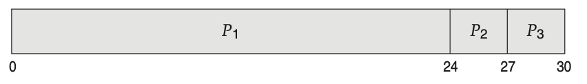
First-Come, First-Served Scheduling
With this scheme, the process that requests the CPU first is allocated the CPU first.
When a process enters the ready queue, its PCB is linked onto the tail of the queue. When the CPU is free, it is allocated to the process at the head of the queue.
On the negative side, the average waiting time under the FCFS policy is often quite long.
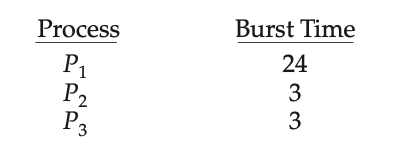
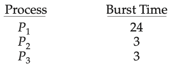
The average waiting time : (0 + 24 + 27) / 3 = 17
The average waiting time : (6 + 0 + 3) / 3 = 3
There is a convoy effect as all the other processes wait for the one big process to get off the CPU. This effect results in lower CPU and device utilization than might be possible if the shorter processes were allowed to go first.
Shortest-Job-First Scheduling
This algorithm associates with each process the length of the process’s next CPU burst. When the CPU is available, it is assigned to the process that has the smallest next CPU burst. If the next CPU bursts of two processes are the same, FCFS scheduling is used to break the tie.
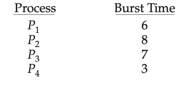
The SJF scheduling algorithm is provably optimal, in that it gives the mini- mum average waiting time for a given set of processes.
The next CPU burst is generally predicted as an exponential average of the measured lengths of previous CPU bursts.
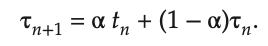
Let tn be the length of the nth CPU burst, and let τn+1 be our predicted value for the next CPU burst. Then, for α, 0 ≤ α ≤ 1, define
The value of tn contains our most recent information, while τn stores the past history. The parameter α controls the relative weight of recent and past history in our prediction. If α = 0, then τn+1 = τn, and recent history has no effect (current conditions are assumed to be transient). If α = 1, then τn+1 = tn, and only the most recent CPU burst matters (history is assumed to be old and irrelevant). More commonly, α = 1/2, so recent history and past history are equally weighted
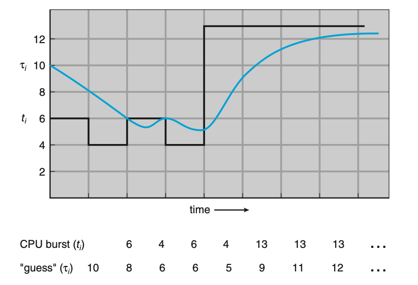
To understand the behavior of the exponential average, we can expand the formula for τn+1 by substituting for τn to find :

The SJF algorithm can be either preemptive or nonpreemptive.
Preemptive SJF scheduling is sometimes called shortest-remaining- time-firs scheduling.
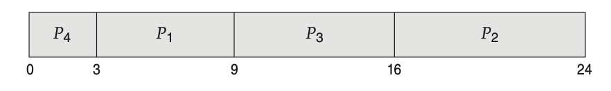
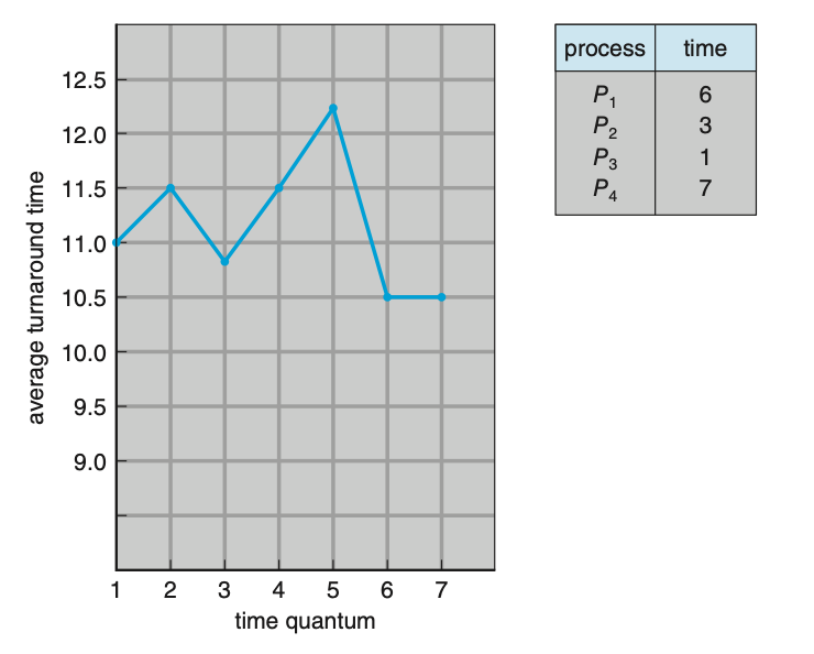
Round-Robin Scheduling
A small unit of time, called a time quantum or time slice, is defined. A time quantum is generally from 10 to 100 milliseconds in length. The ready queue is treated as a circular queue. The CPU scheduler goes around the ready queue, allocating the CPU to each process for a time interval of up to 1 time quantum.
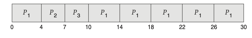
If there are n processes in the ready queue and the time quantum is q, then each process gets 1/n of the CPU time in chunks of at most q time units. Each process must wait no longer than (n − 1) × q time units until its next time quan- tum.
The performance of the RR algorithm depends heavily on the size of the time quantum. At one extreme, if the time quantum is extremely large, the RR policy is the same as the FCFS policy. In contrast, if the time quantum is extremely small (say, 1 millisecond), the RR approach can result in a large number of context switches.
Priority Scheduling
A priority is associated with each process, and the CPU is allocated to the process with the highest priority. Equal-priority processes are scheduled in FCFS order.
In this text, we assume that low numbers represent high priority.
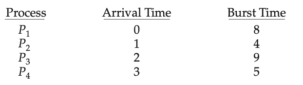
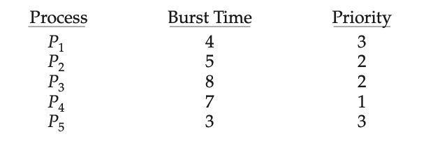
As an example, consider the following set of processes, assumed to have arrived at time 0 in the order P1, P2, · · ·, P5, with the length of the CPU burst given in milliseconds:

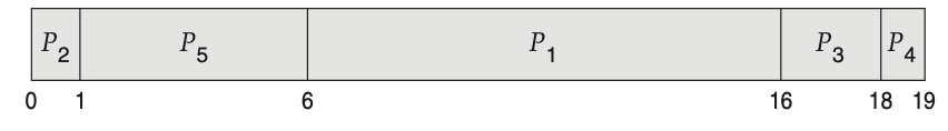
Priority scheduling can be either preemptive or nonpreemptive.
A major problem with priority scheduling algorithms is indefinit block- ing, or starvation.
A solution to the problem of indefinite blockage of low-priority processes is aging.
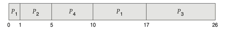
Another option is to combine round-robin and priority scheduling in such a way that the system executes the highest-priority process and runs processes with the same priority using round-robin scheduling.
Multilevel Queue Scheduling
Depending on how the queues are managed, an O(n) search may be necessary to determine the highest-priority process.
There are multiple processes in the highest-priority queue, they are executed in round-robin order.
Separate queues might be used for foreground and background processes, and each queue might have its own scheduling algorithm. The foreground queue might be scheduled by an RR algorithm, for example, while the background queue is scheduled by an FCFS algorithm.
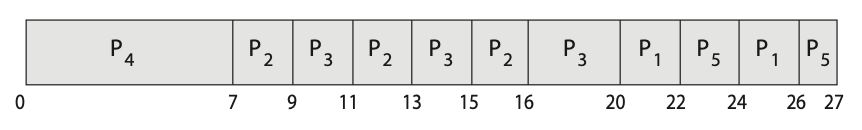
Multilevel Feedback Queue Scheduling
The multilevel feedback queue scheduling algorithm, in contrast, allows a process to move between queues. The idea is to separate processes according to the characteristics of their CPU bursts. If a process uses too much CPU time, it will be moved to a lower-priority queue. This scheme leaves I/O-bound and interactive processes—which are typically characterized by short CPU bursts —in the higher-priority queues. In addition, a process that waits too long in a lower-priority queue may be moved to a higher-priority queue. This form of aging prevents starvation.
An entering process is put in queue 0. A process in queue 0 is given a time quantum of 8 milliseconds. If it does not finish within this time, it is moved to the tail of queue 1. If queue 0 is empty, the process at the head of queue 1 is given a quantum of 16 milliseconds. If it does not complete, it is preempted and is put into queue 2. Processes in queue 2 are run on an FCFS basis but are run only when queues 0 and 1 are empty. To prevent starvation, a process that waits too long in a lower-priority queue may gradually be moved to a higher-priority queue.
In general, a multilevel feedback queue scheduler is defined by the follow- ing parameters:
- The number of queues
- Theschedulingalgorithmforeachqueue
- The method used to determine when to upgrade a process to a higher- priority queue
- The method used to determine when to demote a process to a lower- priority queue
- The method used to determine which queue a process will enter when that process needs service
'CS > 운영체제' 카테고리의 다른 글
| 5.5 Multi-Processor Scheduling (0) | 2023.11.18 |
|---|---|
| 5.4 Thread Scheduling (1) | 2023.11.18 |
| 5.2 Scheduling Criteria (0) | 2023.11.18 |
| 5.1 Basic Concept of CPU Scheduling (0) | 2023.11.18 |
| 4.7 Operating-System Examples (0) | 2023.11.13 |

